My question is how to estimate the observed frequency and its time derivative. The paper states (on page 3) that they were able to estimate these values from Fig. 1, but I was wondering if there was a way to get the exact frequency without having to sort of “eyeball” it from the graph. The actual methods used were not clear to me. (Apologies in advance if the answer is obvious and I’m just missing it!)
I think there’s different ways to answer this question. If by “actual methods”, you mean "how does the LIGO/Virgo/KAGRA collaboration do this, the answer is that we try fitting different waveforms to the data, and see which one fits the best.
For the papers we write, we typically use a Bayesian sampler, like bilby, to try LOTS of different waveforms, in a process called parameter estimation.
Having said all of that, there are a few good papers that show methods for trying to directly extract the f and f_dot from the data. Here are two of my favorites, linked below.
The observed frequency and its time derivative can be estimated from the time-frequency representation of the gravitational wave signal, often referred to as a spectrogram or a Q-transform of the data. This is essentially what is shown in Figure 1 of the paper.
The frequency evolution of a binary black hole merger signal is characterized by a “chirp” - the frequency increases over time as the two black holes spiral closer together and eventually merge. This chirp is visible as a curve in the time-frequency representation.
To estimate the frequency and its derivative at the time of the merger, you would identify the point of highest frequency on this curve (the “peak” of the chirp). The frequency at this point is the observed frequency. The slope of the curve at this point (which can be estimated as the change in frequency over the change in time) is the time derivative of the frequency.
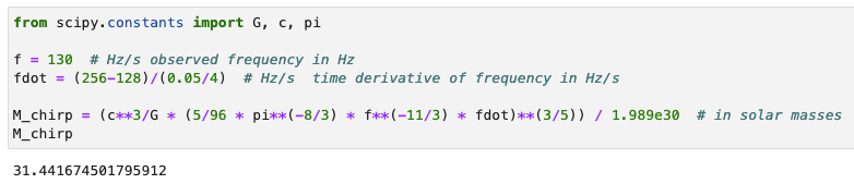
The chirp mass of the system can then be estimated from these values using the following formula:
from scipy.constants import G, c, pi

f = 130  # Hz/s observed frequency in Hz
fdot = (256-128)/(0.05/4)  # Hz/s  time derivative of frequency in Hz/s

M_chirp = (c**3/G * (5/96 * pi**(-8/3) * f**(-11/3) * fdot)**(3/5)) / 1.989e30  # in solar masses
M_chirp
This formula is derived from the post-Newtonian approximation of General Relativity, which describes the evolution of the binary system.
Please note that this is a rough estimate. For a more precise estimation, a full parameter estimation analysis as recommended by @jonah would be performed, which involves matching the observed data against a bank of theoretical waveform templates.
@IPhysReserch Thank you for your clear and detailed response, and the Python code was also helpful.
As a follow up, I wanted to see if I could programmatically retrieve the spectrograms for all events in the GWTC and perform similar calculations as a sort of “toy project” to work on as I learn more about gravitational wave analysis. If you are interested, you can take a look at my notebook here.
However, one of the things I noticed was that not all mergers have the classic “chirp” signal which is very apparent in GW150914, and I was wondering why that was the case. Several events seem to not have any visible signal while others display somewhat irregular shapes. I am sure others who look through the spectrograms for the first time might also wonder about the same thing. What I was able to tell is that the clearest signals were for events with higher SNRs (which obviously makes sense) and higher masses, but I’m curious to know how the parameter estimation gets affected in those cases where almost no signal is visible.
I have directly viewed your notebook from GitHub. Your observation is correct: signals with higher signal-to-noise ratios (SNRs) are more clearly visible in the time-frequency domain under the Q-transform. The strength of parameter estimation within the Bayesian framework is precisely in its ability to quantify this directly from empirical data. It can assess whether a signal is visible relative to the noise. In contrast, signal processing techniques like whitening and time-frequency analysis are not as straightforward, making it challenging to manually filter and capture the most appropriate results to make the signal visible to the naked eye.